TensorFlow2.X学习笔记(6)--TensorFlow中阶API之特征列、激活函数、模型层

一、特征列feature_column

特征列通常用于对结构化数据实施特征工程时候使用，图像或者文本数据一般不会用到特征列。使用特征列可以将类别特征转换为one-hot编码特征，将连续特征构建分桶特征，以及对多个特征生成交叉特征等等。

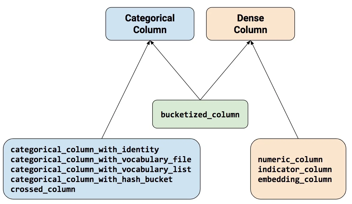
注意：所有的Catogorical Column类型最终都要通过indicator_column转换成Dense Column类型才能传入模型！

numeric_column 数值列，最常用。
bucketized_column 分桶列，由数值列生成，可以由一个数值列出多个特征，one-hot编码。
categorical_column_with_identity 分类标识列，one-hot编码，相当于分桶列每个桶为1个整数的情况。
categorical_column_with_vocabulary_list 分类词汇列，one-hot编码，由list指定词典。
categorical_column_with_vocabulary_file 分类词汇列，由文件file指定词典。
categorical_column_with_hash_bucket 哈希列，整数或词典较大时采用。
indicator_column 指标列，由Categorical Column生成，one-hot编码
embedding_column 嵌入列，由Categorical Column生成，嵌入矢量分布参数需要学习。嵌入矢量维数建议取类别数量的 4 次方根。
crossed_column 交叉列，可以由除categorical_column_with_hash_bucket的任意分类列构成。

示例代码

#================================================================================
# 二，定义特征列
#================================================================================
printlog("step2: make feature columns...")

feature_columns = []

# 数值列
for col in ['age','fare','parch','sibsp'] + [
    c for c in dfdata.columns if c.endswith('_nan')]:
    feature_columns.append(tf.feature_column.numeric_column(col))

# 分桶列
age = tf.feature_column.numeric_column('age')
age_buckets = tf.feature_column.bucketized_column(age, 
             boundaries=[18, 25, 30, 35, 40, 45, 50, 55, 60, 65])
feature_columns.append(age_buckets)

# 类别列
# 注意：所有的Catogorical Column类型最终都要通过indicator_column转换成Dense Column类型才能传入模型！！
sex = tf.feature_column.indicator_column(
      tf.feature_column.categorical_column_with_vocabulary_list(
      key='sex',vocabulary_list=["male", "female"]))
feature_columns.append(sex)

pclass = tf.feature_column.indicator_column(
      tf.feature_column.categorical_column_with_vocabulary_list(
      key='pclass',vocabulary_list=[1,2,3]))
feature_columns.append(pclass)

ticket = tf.feature_column.indicator_column(
     tf.feature_column.categorical_column_with_hash_bucket('ticket',3))
feature_columns.append(ticket)

embarked = tf.feature_column.indicator_column(
      tf.feature_column.categorical_column_with_vocabulary_list(
      key='embarked',vocabulary_list=['S','C','B']))
feature_columns.append(embarked)

# 嵌入列
cabin = tf.feature_column.embedding_column(
    tf.feature_column.categorical_column_with_hash_bucket('cabin',32),2)
feature_columns.append(cabin)

# 交叉列
pclass_cate = tf.feature_column.categorical_column_with_vocabulary_list(
          key='pclass',vocabulary_list=[1,2,3])

crossed_feature = tf.feature_column.indicator_column(
    tf.feature_column.crossed_column([age_buckets, pclass_cate],hash_bucket_size=15))

feature_columns.append(crossed_feature)

二、常用激活函数

tf.nn.sigmoid：将实数压缩到0到1之间，一般只在二分类的最后输出层使用。主要缺陷为存在梯度消失问题，计算复杂度高，输出不以0为中心。

tf.nn.softmax：sigmoid的多分类扩展，一般只在多分类问题的最后输出层使用。

tf.nn.tanh：将实数压缩到-1到1之间，输出期望为0。主要缺陷为存在梯度消失问题，计算复杂度高。

tf.nn.relu：修正线性单元，最流行的激活函数。一般隐藏层使用。主要缺陷是：输出不以0为中心，输入小于0时存在梯度消失问题(死亡relu)。

tf.nn.leaky_relu：对修正线性单元（relu）的改进，解决了死亡relu问题。

tf.nn.elu：指数线性单元。对relu的改进，能够缓解死亡relu问题。

tf.nn.selu：扩展型指数线性单元。在权重用tf.keras.initializers.lecun_normal初始化前提下能够对神经网络进行自归一化。不可能出现梯度爆炸或者梯度消失问题。需要和Dropout的变种AlphaDropout一起使用。

tf.nn.swish：自门控激活函数。谷歌出品，相关研究指出用swish替代relu将获得轻微效果提升。

gelu：高斯误差线性单元激活函数。在Transformer中表现最好。tf.nn模块尚没有实现该函数。

import numpy as np
import pandas as pd
import tensorflow as tf
from tensorflow.keras import layers,models

tf.keras.backend.clear_session()

model = models.Sequential()
# 通过 activation参数指定
model.add(layers.Dense(32,input_shape = (None,16),activation = tf.nn.relu)) 

model.add(layers.Dense(10))
model.add(layers.Activation(tf.nn.softmax))  # 显式添加layers.Activation激活层
model.summary()

# 打印结果：
Model: "sequential"
_________________________________________________________________
Layer (type)                 Output Shape              Param #   
=================================================================
dense (Dense)                (None, None, 32)          544       
_________________________________________________________________
dense_1 (Dense)              (None, None, 10)          330       
_________________________________________________________________
activation (Activation)      (None, None, 10)          0         
=================================================================
Total params: 874
Trainable params: 874
Non-trainable params: 0

三、模型层

1、内置模型层

基础层

Dense：密集连接层。参数个数 = 输入层特征数× 输出层特征数(weight)＋输出层特征数(bias)
Activation：激活函数层。一般放在Dense层后面，等价于在Dense层中指定activation。
Dropout：随机置零层。训练期间以一定几率将输入置0，一种正则化手段。
BatchNormalization：批标准化层。通过线性变换将输入批次缩放平移到稳定的均值和标准差。可以增强模型对输入不同分布的适应性，加快模型训练速度，有轻微正则化效果。一般在激活函数之前使用。
SpatialDropout2D：空间随机置零层。训练期间以一定几率将整个特征图置0，一种正则化手段，有利于避免特征图之间过高的相关性。
Input：输入层。通常使用Functional API方式构建模型时作为第一层。
DenseFeature：特征列接入层，用于接收一个特征列列表并产生一个密集连接层。
Flatten：压平层，用于将多维张量压成一维。
Reshape：形状重塑层，改变输入张量的形状。
Concatenate：拼接层，将多个张量在某个维度上拼接。
Add：加法层。
Subtract：减法层。
Maximum：取最大值层。
Minimum：取最小值层。

卷积网络相关层

Conv1D：普通一维卷积，常用于文本。参数个数 = 输入通道数×卷积核尺寸(如3)×卷积核个数
Conv2D：普通二维卷积，常用于图像。参数个数 = 输入通道数×卷积核尺寸(如3乘3)×卷积核个数
Conv3D：普通三维卷积，常用于视频。参数个数 = 输入通道数×卷积核尺寸(如3乘3乘3)×卷积核个数
SeparableConv2D：二维深度可分离卷积层。不同于普通卷积同时对区域和通道操作，深度可分离卷积先操作区域，再操作通道。即先对每个通道做独立卷即先操作区域，再用1乘1卷积跨通道组合即再操作通道。参数个数 = 输入通道数×卷积核尺寸 + 输入通道数×1×1×输出通道数。深度可分离卷积的参数数量一般远小于普通卷积，效果一般也更好。
DepthwiseConv2D：二维深度卷积层。仅有SeparableConv2D前半部分操作，即只操作区域，不操作通道，一般输出通道数和输入通道数相同，但也可以通过设置depth_multiplier让输出通道为输入通道的若干倍数。输出通道数 = 输入通道数 × depth_multiplier。参数个数 = 输入通道数×卷积核尺寸× depth_multiplier。
Conv2DTranspose：二维卷积转置层，俗称反卷积层。并非卷积的逆操作，但在卷积核相同的情况下，当其输入尺寸是卷积操作输出尺寸的情况下，卷积转置的输出尺寸恰好是卷积操作的输入尺寸。
LocallyConnected2D: 二维局部连接层。类似Conv2D，唯一的差别是没有空间上的权值共享，所以其参数个数远高于二维卷积。
MaxPooling2D: 二维最大池化层。也称作下采样层。池化层无参数，主要作用是降维。
AveragePooling2D: 二维平均池化层。
GlobalMaxPool2D: 全局最大池化层。每个通道仅保留一个值。一般从卷积层过渡到全连接层时使用，是Flatten的替代方案。
GlobalAvgPool2D: 全局平均池化层。每个通道仅保留一个值。

循环网络相关层

Embedding：嵌入层。一种比Onehot更加有效的对离散特征进行编码的方法。一般用于将输入中的单词映射为稠密向量。嵌入层的参数需要学习。
LSTM：长短记忆循环网络层。最普遍使用的循环网络层。具有携带轨道，遗忘门，更新门，输出门。可以较为有效地缓解梯度消失问题，从而能够适用长期依赖问题。设置return_sequences = True时可以返回各个中间步骤输出，否则只返回最终输出。
GRU：门控循环网络层。LSTM的低配版，不具有携带轨道，参数数量少于LSTM，训练速度更快。
SimpleRNN：简单循环网络层。容易存在梯度消失，不能够适用长期依赖问题。一般较少使用。
ConvLSTM2D：卷积长短记忆循环网络层。结构上类似LSTM，但对输入的转换操作和对状态的转换操作都是卷积运算。
Bidirectional：双向循环网络包装器。可以将LSTM，GRU等层包装成双向循环网络。从而增强特征提取能力。
RNN：RNN基本层。接受一个循环网络单元或一个循环单元列表，通过调用tf.keras.backend.rnn函数在序列上进行迭代从而转换成循环网络层。
LSTMCell：LSTM单元。和LSTM在整个序列上迭代相比，它仅在序列上迭代一步。可以简单理解LSTM即RNN基本层包裹LSTMCell。
GRUCell：GRU单元。和GRU在整个序列上迭代相比，它仅在序列上迭代一步。
SimpleRNNCell：SimpleRNN单元。和SimpleRNN在整个序列上迭代相比，它仅在序列上迭代一步。
AbstractRNNCell：抽象RNN单元。通过对它的子类化用户可以自定义RNN单元，再通过RNN基本层的包裹实现用户自定义循环网络层。
Attention：Dot-product类型注意力机制层。可以用于构建注意力模型。
AdditiveAttention：Additive类型注意力机制层。可以用于构建注意力模型。
TimeDistributed：时间分布包装器。包装后可以将Dense、Conv2D等作用到每一个时间片段上。

2、自定义模型层

如果自定义模型层没有需要被训练的参数，一般推荐使用Lamda层实现。
如果自定义模型层有需要被训练的参数，则可以通过对Layer基类子类化实现。

Lamda层

Lamda层由于没有需要被训练的参数，只需要定义正向传播逻辑即可，使用比Layer基类子类化更加简单。

Lamda层的正向逻辑可以使用Python的lambda函数来表达，也可以用def关键字定义函数来表达。

import tensorflow as tf
from tensorflow.keras import layers,models,regularizers

mypower = layers.Lambda(lambda x:tf.math.pow(x,2))
mypower(tf.range(5))

Layer层

class Linear(layers.Layer):
    def __init__(self, units=32, **kwargs):
        super(Linear, self).__init__(**kwargs)
        self.units = units

    #build方法一般定义Layer需要被训练的参数。    
    def build(self, input_shape): 
        self.w = self.add_weight(shape=(input_shape[-1], self.units),
                                 initializer='random_normal',
                                 trainable=True)
        self.b = self.add_weight(shape=(self.units,),
                                 initializer='random_normal',
                                 trainable=True)
        super(Linear,self).build(input_shape) # 相当于设置self.built = True

    #call方法一般定义正向传播运算逻辑，__call__方法调用了它。    
    def call(self, inputs): 
        return tf.matmul(inputs, self.w) + self.b

    #如果要让自定义的Layer通过Functional API 组合成模型时可以序列化，需要自定义get_config方法。
    def get_config(self):  
        config = super(Linear, self).get_config()
        config.update({'units': self.units})
        return config

linear = Linear(units = 8)
print(linear.built)
#指定input_shape，显式调用build方法，第0维代表样本数量，用None填充
linear.build(input_shape = (None,16)) 
print(linear.built)

linear = Linear(units = 16)
print(linear.built)
#如果built = False，调用__call__时会先调用build方法, 再调用call方法。
linear(tf.random.uniform((100,64))) 
print(linear.built)
config = linear.get_config()
print(config)

tf.keras.backend.clear_session()

model = models.Sequential()
#注意该处的input_shape会被模型加工，无需使用None代表样本数量维
model.add(Linear(units = 16,input_shape = (64,)))  
print("model.input_shape: ",model.input_shape)
print("model.output_shape: ",model.output_shape)
model.summary()

# 打印结果：
model.input_shape:  (None, 64)
model.output_shape:  (None, 16)
Model: "sequential"
_________________________________________________________________
Layer (type)                 Output Shape              Param #   
=================================================================
linear (Linear)              (None, 16)                1040      
=================================================================
Total params: 1,040
Trainable params: 1,040
Non-trainable params: 0